Running MPL for Windows

This page is produced from the introductionary material that comes with MPL for Windows.

Start MPL

To start MPL for Windows select it from the Start Menu that appears along the bottom of the Windows 95/98 desktop. The MPL start menu entry is shown here in Figure 1.

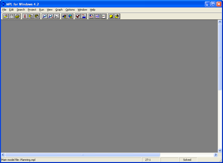
When you start MPL in stand-alone mode the main window appears. From it you can select all the actions you wish MPL to do.

The main window consists of the title bar at the top, the main menu, the toolbar, the work area and the status line at the bottom. The menus and toolbar provides you with easy access to all the features that MPL offers in the user-friendly Windows environment. The toolbar allows you to choose the most commonly used menu commands quickly by pressing a button.

Using the Model Editor

To create a new model choose New from the File menu. MPL will then open an empty editor window with the name <untitled>. If you want to open an existing model file choose the Open command from the File menu. The standard Open File dialog box like the one shown below will then be displayed.

In the middle of the dialog box is a list of all the files that are in the current folder. To open a file, select it from the list of files and press the Open button. You can also open the file directly by double-clicking on it in the list of files. Alternatively, you can enter the filename in the File name input box below the list and then press the Open button.

The name of the current folder is shown in the Look in input box at the top of the dialog. If the file you want to open is in a different folder, you can press the down arrow at the right of the Look in input box to navigate through the directory tree. Select the folder name you want to go to and the list of files below will reflect the contents of the new folder.

After you have opened a file, a model editor window opens where you can type in and edit your model. This editor works like any other standard Windows editor, allowing you to use the mouse, arrow keys, or the scroll bars to move around the file. If you make a mistake while entering your model you can use the Undo command in the Edit menu to correct it.

If you need to copy text either within the editor or between different editor files you can use the standard Windows clipboard operations. To copy text to the clipboard, you first select the text using the mouse, then you copy it to the clipboard using the Copy command from the Edit menu. If you want to move the text instead of copying it, you can use the Cut command. After you have copied the text to the clipboard, you move the cursor where you want to place the text and use the Paste command to place it.

If you need to search for text in your model file, you can use the Find command from the Search menu. This will bring up the Find dialog box where you enter the text you want to search for and set options that control how MPL searches for the text. If you need to replace the text in the model file use the Replace command in the Find menu.

When you are ready to save your model file you can use either the Save command or the Save As command in the File menu. Use the Save command when you want to save the file using the current name. When you want to save the model file under a different name use the Save As command.

Solve the Model

After you have entered your model in the model editor choose Solve from the Runmenu to optimize the model. While optimizing MPL displays a status window that provides you with information on the solution progress as shown here below:

While MPL reads the model file, the status window displays the name of the file being read, the number of lines read so far, the number of variables and constraints in the model, and how much memory has been used. While the optimizer is solving the model, the number of iterations and the value of the objective function are shown.

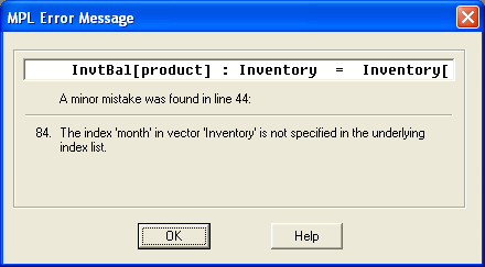
If MPL finds a mistake or an error in the model, an error message will be displayed. It shows the erroneous line in the model with short explanation in plain language of what the problem is. The cursor will automatically be positioned at the error in the model file, with the mistake highlighted.

View the Solution Results

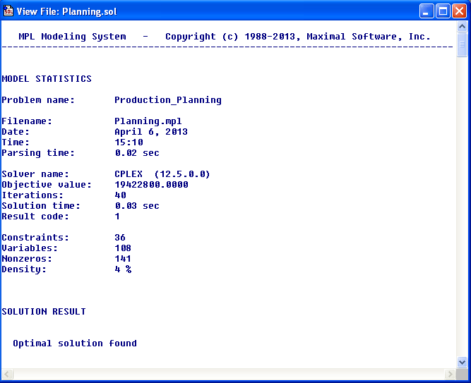
After the model has been solved MPL will generate a solution file. You can select the Filescommand in the View menu to display the solution file in a view window.

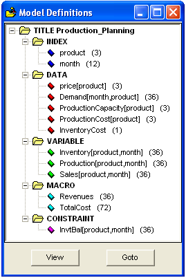
The view window stores the file in memory allowing you to quickly browse through the solution on the screen using the scroll bars. You can also use various commands in the View menu to view other generated files, the model statistics, and the solution values. The Model Definitions window also allows you to view all the defined items in the model in an easy to use hierarchical tree structure.

Each branch in the tree corresponds to a section in the model. You can expand and collapse each branch to show only the elements you are interested in. Double-lick on any item to get the solution values for that item. You can leave the Model Definitions window open for the duration of the MPL session since it will be automatically updated every time you run your model.

Display Graph of the Matrix

MPL also allows you to display a graph of the matrix nonzero elements, by choosing Matrix from the Graph menu.

The positive numbers are shown using blue dots and negative numbers using red dots. If the nonzero is either 1 or -1 the dot will displayed using a little bit brighter color.

You can use the mouse to zoom into the matrix. Place the cursor in the upper-left corner of the part of the matrix you want to zoom into. Hold the left mouse button down and drag the mouse down and to the right. This will draw a box that shows the area that will be zoomed. When the box is the correct size release the left mouse button to zoom.

You can repeat the zoom several times until you reach the spreadsheet view. This will allow you to see the actual values and the names of each cell in the matrix. You can also reach the spreadsheet view by just clicking with the left mouse button on the part of matrix you want to see. To move around use the arrow keys. To zoom back click the right mouse button.

You can also display a graph of the objective function values for each iteration by choosing Objective Function from the Graph menu. The graph will show the objective function values with a dark red line and the amount of infeasibilities for Phase 1 iterations with a green line. For integer problems the graph will show the objective function value for each node and the best integer solution value found so far using blue lines. This graph is only available when the model has been solved using Windows/DLL solvers.

Change Options Settings

MPL offers a range of options dialog boxes in the Options menu that allow you to change various default settings and preferences for MPL.

For example, to change various options for the MPL integrated environment choose Environment from the Options menu. If you want to change the settings for the MPL language or the database connection choose the MPL Language or Database respectively from the Options menu

If you want to change the contents and various options for the solution file, choose Solution File from the Options menu. This dialog box allows you among other things change the solution filename, set the number of decimal places, and decide what the solution file should contain.

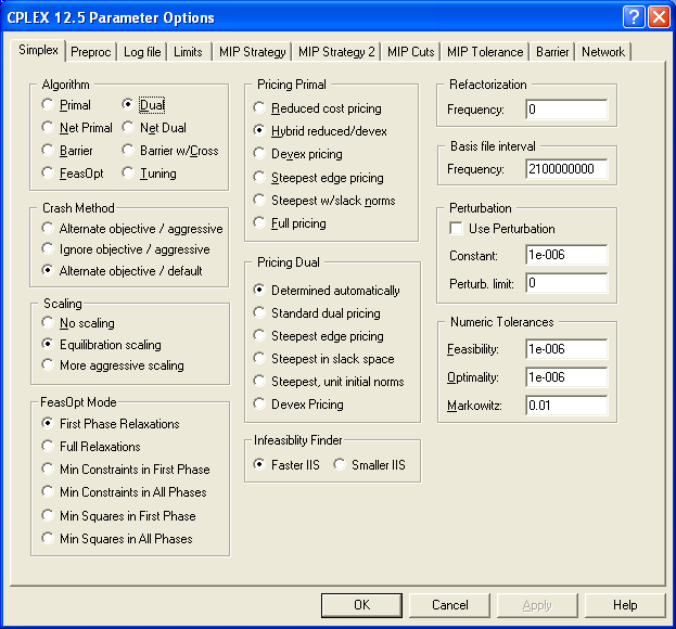
MPL offers a number of dialog boxes that allow you to change option parameters for supported solvers. Which options you can set depends on the solver you are using. The CPLEX optimizer, for example, offers seven different options dialog boxes, while XA options are set through a special text edit dialog box. For example, to display the simplex algorithmic options for CPLEX, choose CPLEX Parameters | Simplex from the Options menu.

To change which solvers are shown in the Run menu choose Solver Menu from the Option menu. This will display the Solver Menu Setup dialog box, containing a list of all the solvers supported by MPL. To let the Run menu reflect which solvers you have installed on your machine, double-click on the solver to either add or remove it from the menu. If you need to change some of the setup options for a solver, including where it resides on the hard-disk, press the Edit button.